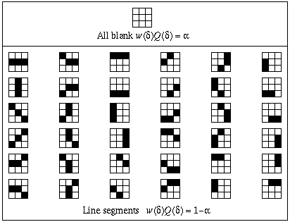
The Dictionary

The dictionary is the set of all neighborhood patterns for which wQ is not equal to zero and represents some knowledge about the structure of the data. For images containing thin objects, we make the following assumptions about the data:

• the image consists of neighborhoods containing all blanks or a portion of a thin object
• all neighborhoods containing a portion of a thin object have the same wQ
• all other neighborhoods have wQ = 0

The figure below shows a dictionary suitable for restoring thin lines in two-dimensional images. The neighborhood size is 3 by 3 giving a total of 512 possible neighborhood patters. The dictionary contains only 37 entries for which wQ is not zero.

Figure 2: A dictionary of 3 by 3 neighborhoods suitable for restoration of thin lines.

For larger two-dimensional neighborhoods, and especially for three-dimensional ones, generation of a dictionary is too complicated a task to be done manually. Our algorithm to generate dictionaries for thin line restoration works as follows:

1. establish a Cartesian coordinate system centered on a neighborhood
2. assume always that there is an all blank neighborhood in the dictionary
3. to generate a single neighborhood containing a line segment, compute the distance between each pixel and the segment. If that distance is less than 1/2 then assume the pixel is a one, otherwise assume that pixel is a zero.
4. generate the complete dictionary by applying the above step for a complete range of segment orientations and distance from the central pixel.
5. discard neighborhoods from the dictionary that:
   • are redundant, i.e., occur elsewhere in the dictionary,
   • have too few ones, and
   • have both a row and a column with more than a single one. Avoids neighborhoods that look like:
     

The above algorithm extends easily to three-dimensional neighborhoods and thin sheet restoration.

Computational Efficiency

In the above table, there are only 37 neighborhoods in the dictionary and the restoration is fast. However, as the neighborhood size and number of dimensions increases the restoration can become too slow to be practical.

An analysis of the algorithm shows that the vast majority of the computation is in the summation of norms in the probability distribution phi. We have optimized the speed of computation by recognizing that almost every entry in the dictionary is nearly identical to at least one other. It is then faster to compute the sum by adjusting a previously computed sum for a similar neighborhood than it is to compute the sum from scratch.

Figure 3: Minimum spanning tree for computation of sums for dictionary in Figure 2.

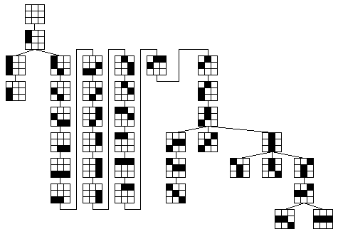
To optimize this approach we represent the dictionary as a graph where each node is a dictionary entry and there is an edge between every pair of nodes. We then assign a weight to each edge equal to the number of pixel differences between the two nodes it connects, and compute a minimum spanning tree. As a result, computing the sums during a depth-first traversal of the tree minimizes the computation. For example, Figure 3 shows the tree derived for the dictionary in Figure 2. A traversal of the tree requires only 106 additions in computing the norms at each image site while 296 are required for the brute force approach. The savings are not that great for such a small dictionary, but the change becomes essential to apply the method with large neighborhoods, especially in three dimensions. For example, we observed better than a 20-fold improvement for a two-dimensional 11 by 11 neighborhood.